Blog
Uncertainties in IB Physics: error bars, gradients and propagation
Uncertainties turn a lab number into a result you can defend. This guide covers absolute, fractional and percentage uncertainty, propagation, rounding, error bars, and how to get the uncertainty in a gradient and intercept from a graph, with worked examples and the mistakes that cost marks.
By Ejaz Ahmad · 21 October 2026 · 9 min read
- Propagation
- Error bars
- Gradient uncertainty
- Exams and IA
An answer of "9.9 m s-2" tells a reader very little. An answer of "9.9 ± 0.7 m s-2" tells them how far to trust it and whether it agrees with 9.81. That is why uncertainty work appears in short exam questions, in data-analysis questions and in the Physics IA. The good news is that the rules are few and mechanical.
Convention varies a little between schools and exam questions, so use the method your teacher and the question ask for. Check the formulas your data booklet gives you, see our Physics data booklet guide, and learn the rest.
Absolute, fractional and percentage uncertainty
Every measurement has the form value ± uncertainty. The three ways of stating the uncertainty are linked:
| Type | Definition | Example for 2.50 ± 0.05 cm |
|---|---|---|
| Absolute | Same unit as the measurement | 0.05 cm |
| Fractional | absolute ÷ value | 0.05 ÷ 2.50 = 0.02 |
| Percentage | fractional × 100% | 2% |
For a single reading, a common school rule is to take half the smallest division on an analogue scale, and the smallest division on a digital display. For repeated readings, half the range (maximum minus minimum) is a usual estimate. Use whichever your class has been taught and say which one you used.
Propagating uncertainties: the three rules
When you calculate a quantity from measurements, their uncertainties combine. Learn three rules.
Sums and differences: add absolute uncertainties
Two lengths: 12.0 ± 0.2 cm and 8.5 ± 0.2 cm. The sum is 20.5 ± 0.4 cm. The difference of 25.4 ± 0.3 cm and 18.1 ± 0.3 cm is 7.3 ± 0.6 cm. Notice that a difference of two similar numbers has a large fractional uncertainty, about 8% here, even though each input was about 1%.
Products and quotients: add percentage uncertainties
A trolley has mass 0.250 ± 0.005 kg (2.0%) and acceleration 3.2 ± 0.1 m s-2 (3.1%). Force F = ma = 0.800 N. Percentage uncertainty is 2.0 + 3.1 = 5.1%, which is 0.04 N. So F = 0.80 ± 0.04 N.
For a quotient, do exactly the same. A speed v = d/t with d = 1.50 ± 0.02 m (1.3%) and t = 0.82 ± 0.02 s (2.4%) gives v = 1.83 m s-1 with 3.7%, so v = 1.83 ± 0.07 m s-1.
Powers: multiply the percentage uncertainty by the power
A circle has radius 2.5 ± 0.1 cm (4%). The area πr² has uncertainty 2 × 4 = 8%. Area = 19.6 cm², and 8% of that is 1.6 cm², so area = (20 ± 2) cm². A volume that depends on r³ would carry 12%. The same rule works for roots: a square root halves the percentage.
Quick check
Which rule applies?
- Adding or subtracting: add absolute uncertainties.
- Multiplying or dividing: add percentage uncertainties.
- Raising to a power n: multiply the percentage uncertainty by n.
- Constants such as 2 or π carry no uncertainty and do not change the percentage.
From my classes at Photon Academy: the most frequent slip is mixing the two types, adding an absolute uncertainty to a percentage. Convert everything to the same type before you add.
Significant figures and rounding
The uncertainty tells you how many digits are worth keeping. State the uncertainty to one significant figure (two only if its leading digit is 1 and you want the extra care), then round the value to the same decimal place.
- 9.8765 ± 0.3 becomes 9.9 ± 0.3.
- 0.80 ± 0.041 becomes 0.80 ± 0.04.
- Wrong: 9.8765 ± 0.3, with too many digits, or 10 ± 0.3, with too few.
Round only at the end. Keep extra digits through the working so that rounding does not add its own error.
Error bars and the best-fit line
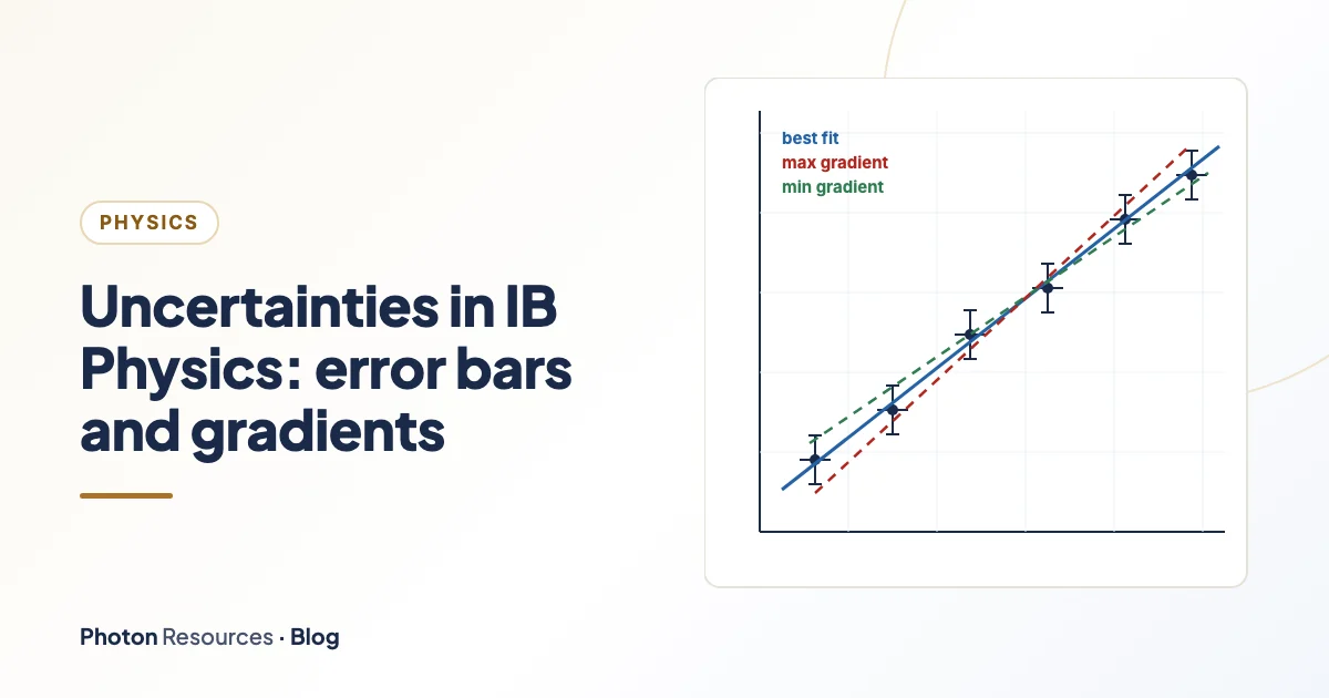
An error bar shows the uncertainty on a plotted point. Vertical bars show the uncertainty in y and horizontal bars the uncertainty in x. If one is too small to draw at your scale, say so. A good best-fit line passes through most of the error bars, with points above and below it and does not have to pass through the origin or through any particular point.
If you have the freedom to choose the graph, choose one that gives a straight line. For a pendulum T² = (4π²/g) L, so the gradient is 4π²/g.
Uncertainty in the gradient and intercept
The method uses two extra lines. The steepest line is the line of greatest gradient that still passes through all the error bars. The shallowest line is the one with the least. Take half the difference of their gradients.
- Best-fit gradientFrom the graph: 3.99 s² m-1.
- Maximum and minimum gradientsSteepest 4.29 and shallowest 3.69 s² m-1.
- Uncertainty(4.29 − 3.69) ÷ 2 = 0.30. So gradient = 4.0 ± 0.3 s² m-1.
- Use itg = 4π² ÷ gradient = 9.87 m s-2. The gradient is 7.5% uncertain, so g has 7.5%, which is 0.74. Then g = 9.9 ± 0.7 m s-2, and 9.81 lies inside that range.
For the intercept, do the same with the intercepts of the two extreme lines. Here the best line meets the y-axis at about 0.01 s², and the extreme lines give about −0.18 and +0.18, so the intercept is 0.01 ± 0.18 s². Since zero lies inside, there is no evidence of a significant offset. For this experiment, you would expect zero, so that is a useful check on systematic error.
Random and systematic errors
Random errors come from limits in reading, timing or changing conditions. They are reduced by repeating and averaging, and they show up as scatter and as error bars. Systematic errors push every reading the same way, such as a ruler with a worn end or a meter that reads 0.02 V when nothing is connected. Repetition will not remove them. On a graph a systematic error often appears as an intercept that should be zero but is not.
When you evaluate, name the specific source, say whether it is random or systematic, and say which way it changes your result. In my experience this is where IA marks are won or lost: "human error" says nothing, while "starting the stopwatch about 0.2 s after release, making each T too small" says everything. See the Physics IA criteria for how this is assessed, and our Physics IA guide for planning.
Common exam and IA mistakes
- Reporting the uncertainty to too many figures. Keep to one significant figure.
- Adding percentages for sums. Percentages are for products, quotients and powers only.
- Forgetting the power. A cube needs 3 times the percentage.
- Drawing the best-fit line through the origin when the data does not go there.
- Joining the dots instead of drawing one smooth best-fit line.
- Using the whole range as the uncertainty when half the range was asked for.
- Using the minimum and maximum lines that ignore the error bars at the ends.
- Missing the units in the final answer or the gradient.
Another habit worth building: always compare your result with the accepted value using the uncertainty, in a sentence such as "the accepted value lies within my range, so the result is consistent".
Where to go next
For official background, the NIST guide to uncertainty of measurement gives clear definitions and examples, and the BIPM Guide to the Expression of Uncertainty in Measurement (JCGM 100) is the international reference. To practise collecting data from a launcher, try the PhET Projectile Data Lab. For course context, this article explains what changed in the IB Physics course from 2025.
Uncertainty questions sit inside both IB Physics HL and IB Physics SL. Practise them in short sets, so the three rules become automatic.
Practise it
Make uncertainty marks routine
Work through Physics questions at Foundation, Core, Exam and Challenge level, with two topics in every course free.